Geodesics on \({SL}(n)\) with the Hilbert-Schmidt metric, and one application to fluids
Willie Wai Yeung Wong wongwwy@math.msu.edu Michigan State University
Slides available : https://slides-n-notes.qnlw.info
Credits page
Joint work with:
Audrey Rosevear, Amherst College
Samuel Sottile, Michigan State University
Support by NSF through the SURIEM (2020) summer REU site at MSU.
Paper to appear in La Matematica ; arXiv:2101.09266 .
Audrey will present a poster on this at JMM2022; do stop by and say hi!
Outline
Set-up
Physics
Geometry; prior results
Our results
Application; what's next?
Dramatis personae
$M(n)$ — space of $n\times n$ real matrices
$S(n)$ — symmetric elements of $M(n)$
$SL(n)$ — determinant 1 elements of $M(n)$
$SO(n)$ — elements of $SL(n)$ satisfying $A^T = A^{-1}$
$\mathring{S}_+(n)$ — positive definite elements of $S(n) \cap SL(n)$
$\mathfrak{sl}(n)$ — trace 0 elements of $M(n)$
$\mathfrak{so}(n)$ — anti-symmetric elements of $M(n)$
$\langle A, B\rangle := \mathrm{tr}(AB^T)$ — Hilbert-Schmidt inner product on $M(n)$
Hilbert-Schmidt metric on $SL(n)$
$M(n)$ with $\langle A,B\rangle$ $\qquad\cong\qquad$ $\mathbb{R}^{n\times n}$ with standard metric.
$SL(n)$ is a co-dimension 1;
Not bi-invariant!
The Question
What is the geometry of this Riemannian manifold?
Geodesic completeness? — ✓
Existence / stability of bounded geodesics?
Asymptotic behavior and stability of unbounded geodesics?
Why emphasis on geodesics?
Rigid Body
Illustration: motion of rigid body with movement and rotation.
Rigid Body
Initial/reference body: \(\quad \Omega\Subset\mathbb{R}^n\)
Configuration at time \(t\): $\quad x(t) + A(t)\cdot\Omega; \qquad x(t)\in \mathbb{R}^n, \quad A\in SO(n)$
Total kinetic energy: \[ \int_{\Omega} |x'(t) + A'(t)y|^2 ~\mathrm{d}y = \mathrm{vol}(\Omega) |x'(t)|^2 + \mathrm{tr}\left( A'(t) I_\Omega A'(t)^T \right)\]
Moment of inertia: \(\quad \displaystyle I_\Omega = \int_\Omega y y^T ~ \mathrm{d}y\)
For write-up with more details: click here .
Action Principle
\[ S = \int \left[ \mathrm{vol}(\Omega) |x'(t)|^2 + \mathrm{tr}\left( A'(t) I_\Omega A'(t)^T \right) \right] ~dt\]
The integrand defines a positive definite quadratic form on the tangent space of $\mathbb{R}^n\times SO(n)$
Solutions are geodesics w.r.t. this Riemannian metric.Note that the metric given by $I_\Omega$ is not the bi-invariant metric on $SO(n)$.
Motion on $\mathbb{R}^n$ decouples from motion on $SO(n)$.
Affine Motion
Allow the body to also deform linearly but preserving volume.
Swap $SO(n)$ with $SL(n)$.
Everything else the same: $I_\Omega$ induces a Riemannian metric on $SL(n)$ which determines the trajectories.
Why do we only care when $I_\Omega = \mathrm{Id}_n$?
Incompressible Fluids
Allow the body to arbitrarily deform, but preserving infinitesimal volume.
Replace $SO(n)$ by the group(oid) of volume preserving diffeomorphisms.
For fluid flow inside a fixed domain $\Omega$: Euler-Arnol'd equations.
Free boundary problem: requires boundary conditions.
At any fixed time: fluid pressure is constant along (moving) boundary.
Relating affine motion to fluid motion
$SL(n)$ is a subgroup of the group of volume preserving diffeos of $\mathbb{R}^n$.
Boundary conditions satisfied by $SL(n)$ geodesic $\iff$ under the Riemannian metric induced by the geometry of $\Omega$, $SL(n)$ is totally geodesic.
Theorem . This holds iff $\Omega$ is a round ball (and hence $I_\Omega = \mathrm{Id}_n$).
3. Geometry; prior results
Discrete symmetry
\(A \to A^T\) is isometry of \(M(n)\), and fixes \(SL(n)\), so is isometry on \(SL(n)\).
Lemma . $S(n)\cap SL(n)$ is totally geodesic in \(SL(n)\).
Corollary . $\mathring{S}_+(n)$ is totally geodesic in \(SL(n)\).
Continuous symmetries
\(SO(n)\) acting on \(M(n)\) by matrix multiplication is isometric & fixes \(SL(n)\)
Distinct left and right actions!
Generate a total of \(n(n-1)\) Killing vector fields
Physical interpretation: $\quad$ angular momentum and vorticity
Conjugate action: $A \mapsto OAO^{-1}$ (fixes $\mathring{S}_+(n)$)
Composite action: $A \mapsto OAO$ (not faithful)
Polar decomposition
Every $A\in SL(n)$ has a unique factorization as $OP$ (or $PO$): $
\begin{cases} O\in SO(n) \newline P\in \mathring{S}_+(n)\end{cases}$
$SL(n)$ foliated by cosets
So the geodesics are easy to describe, right?
Problem : Left actions generate right-invariant vector fields and vice versa
... so even with our conserved quantities, the motions on the two factors do not split.
$n = 2$ is special: analysis
Motion is completely integrable: $\dim(SL(2)) = 3$ and conservation of
Energy
Angular momentum
Vorticity
Used in Roberts-Shkoller-Sideris (CMP 2020) where geodesics are fully classified.
Will return to this classification a bit later.
$n = 2$ is special: geometry
$SL(2)$ is a warped product $\mathring{S}_+(2) \times_f \mathbb{S}^1$
Use the composite $A\mapsto OAO$ action
double cover of $SL(2)$ by $\mathring{S}_+(2) \times_f SO(2)$.Use $SO(2) = U(1)$ and "take square roots"
$SO(2)$ is abelian:
Composite $OAO$ action is orthogonal to cosets of polar decomposition
Conjugate $OAO^{-1}$ action is tangent to cosets
Decompose as integrable motion on $\mathring{S}_+(2)$ plus fibre motion.
(Private communication from Ben Schmidt)
Definitions
Throat
Call $SO(n)\subsetneq SL(n)$ the "throat": it describes the points closest to the origin in $M(n)$.
Second fundamental form
Sign convention: $II(X,X) \gt 0$ if it curves away from the origin.
Second f.f. defined via normal pointing away from origin of \(M(n)\).
Geodesic equation
Let $X,Y\in T_A SL(n)$, then \[ II(X,Y) = \frac{\mathrm{tr}(A^{-1}X A^{-1}Y)}{|A^{-1}|} \] and the geodesic equation reads
\[ \ddot{A} = \frac{ \mathrm{tr}( A^{-1} \dot{A} A^{-1} \dot{A})}{\mathrm{tr}(A^{-1} A^{-T})} A^{-T}.\]
$n = 2$ geodesic classification
The only bounded geodesic orbits the throat
There exists semi-bounded geodesics converging to the throat
All unbounded geodesics are "asymptotically linear" ($II(\dot{\gamma},\dot{\gamma}) \to 0$)
How much of these survive in higher dimensions?
$n = 3$ prior results
Analyses of some special explicit solutions and their asymptotics
Sideris (ARMA 2017)
$n$-independent prior results
Virial Identity : let $A: t\to M(n)$ a $SL(n)$-geodesic
\[ \frac{d^2}{dt^2} |A|^2 = \frac{|\dot{A}|^2}{|A|} + \frac{n}{|A|^2} II(\dot{A}, \dot{A}).\]Proposition : if additionally $A$ is such that $II(\dot{A}, \dot{A}) \gt 0$ for all $t \gt t_0$, then $A$ is unbounded and asymptotically linear.
Sideris (ARMA 2017)
Higher dimensions are more curvy
Theorem. $SL(2)$ has bounded sectional curvature.Theorem. When $n \geq 3$, given $A\in SL(n)$ and $W\subset T_A SL(n)$ a plane, denote by $k(W)$ its sectional curvature. Then:
$k(W) \leq |A^{-1}|^2$ for all $(A,W)$;
There exists a sequence $(A_i, W_i)$ with
(Remark : the function $A\mapsto |A^{-1}|$ is proper.)
Linear solutions are linearly stable
Linear solutions : those whose images are lines in $M(n)$. Linear stability : Jacobi fields along such curves grow at most linearly.Key step: showing for such $A(t)$ the quantity
\[ \left| \mathrm{Riem}(\dot{A}, J, \dot{A}, K) \right| \lesssim \frac{|J|~ |K|}{(1 + t^4)}. \]
Bounded geodesics abound in $n \geq 4$
Theorem. When $n = 2m \geq 4$, for every $\eta \geq |\mathrm{Id}|$, there exists a bounded geodesic $A(t)$ with $|A(t)| \equiv \eta$.In fact, we can write $A(t) = A_0 \exp (Ct)$ with $A_0 \in \mathring{S}_+(n)$ and $C\in \mathfrak{so}(n)$.
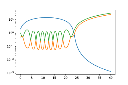
Remark : these are the only "non-linear" "exponential" solutions.Physical picture: Stationary fluid solution; an ellipsoid with "paired" axes, spinning separately in each plane.When the rotational speeds are not "tuned", the solutions remain bounded, but pulsates.
Numerical simulation for $n = 6$, for generic data when axes are paired; plots are the three semi-major axial lengths.
Refinement of Virial argument
\[ \frac{d^2}{dt^2} |A|^2 = \frac{|\dot{A}|^2}{|A|} + \frac{n}{|A|^2} II(\dot{A}, \dot{A}).\]
Lemma . When $n = 2$, we have $\frac{d^2}{dt^2} |A(t)|^2 \leq 0 \implies |A(t)| = |\mathrm{Id}|$.
Corollary . All geodesics except for the throat rotation are unbounded.
Emphatically false when $n \geq 3$.
Virial revisited
Theorem. [sufficient conditions for unboundedness]
Solution is tangent to $\mathring{S}_+(n)$ (or another coset)
Solution has vanishing total angular momentum
Solution has vanishing total vorticity
New formulation of equations
Given solution $A(t)$, define
\[ \beta = A^{-1}A^{-T}, \quad \omega = A^T \dot{A} + \dot{A}^T A, \quad \zeta = A^T \dot{A} - \dot{A}^T A \]
$\beta$: "square" of the "radial component" in polar decomposition
$\omega$: "radial" velocity
$\zeta$: "angular" velocity
Above is the vorticity version; angular momentum version moves the transpose to the other factor.
Cannot do both simultaneously.
New formulation of equations
Solves problem with Killing vector field not pointing in the fibre direction.
\begin{align*}
\frac{d}{dt} \beta & = -\beta \omega \beta \newline
\frac{d}{dt}\omega & = \frac12(\omega + \zeta)^T\beta(\omega + \zeta) + \underbrace{\frac{\mathrm{tr}\omega\beta\omega\beta}{2\mathrm{tr}\beta}}_{\geq 0} I + \underbrace{\frac{\mathrm{tr}\zeta\beta\zeta\beta}{2\mathrm{tr}\beta}}_{\leq 0} I \newline
\frac{d}{dt}\zeta &= 0
\end{align*}
Compatibility condition: $\quad \mathrm{tr}\beta\omega = 0$.
Preserves "block diagonal structure"
Block diagonal solutions
Assume $\beta, \omega,\zeta$ decompose into $2\times 2$ blocks (with one $1\times 1$ block when $n$ is odd) along the diagonal.
A boundedness criterion
Theorem . Let $n$ be even. If the initial data of $\beta,\omega$ are built from $2\times 2$ blocks that are pure-trace, and if $\zeta$ has no vanishing bocks, then the solution is bounded.
When $n = 2$, hypothesis only possible with rotation at throat.
"Swirling and shear flows"
Theorem . If the initial data has the form
\[ \beta_0 = \begin{pmatrix} b_1 \mathrm{Id}_{2m} \newline & b_2 \mathrm{Id}_{n - 2m}\end{pmatrix}, \quad \omega_0 = \begin{pmatrix} w_1 \mathrm{Id}_{2m} \newline & w_2 \mathrm{Id}_{n-2m} \end{pmatrix} \]
and writing $\varepsilon$ for the antisymmetric $2\times 2$ matrix
\[ \zeta_0 = \begin{pmatrix} z (\underbrace{\varepsilon \oplus \cdots \oplus \varepsilon}_{m \text{ copies}}) \newline & 0 \end{pmatrix};\]
then the corresponding solution is unbounded, and asymptotically linear.
Sideris [ARMA 2017] described $n = 3$ and $m = 1$ with explicit integration
Further generalization?
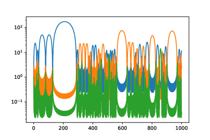
Numerical simulation of a generalized swirling and shear flow with three sets of axes, instead of two.
5. Application; what's next?
Asymptotically linear solutions can be unstable
Let $A(t)$ be a swirling and shear flow: we can show that $II(\dot{A}, \dot{A})$ is eventually positive.
So $A(t)$ is "asymptotically linear"
"Small perturbations"
\[ \zeta_0 = \begin{pmatrix} z (\underbrace{\varepsilon \oplus \cdots \oplus \varepsilon}_{m \text{ copies}}) \newline & 0 \end{pmatrix} \Longrightarrow \begin{pmatrix} z (\underbrace{\varepsilon \oplus \cdots \oplus \varepsilon}_{m \text{ copies}}) \newline & \delta (\varepsilon \oplus \cdots \oplus \varepsilon) \end{pmatrix} \]
Non-vanishing rotation $\implies$ motion is bounded
Connection to fluids
Bounded motions must enter regime with negative second fundamental form.
Physical instability : Rayleigh-Taylor. (Require pressure just inside the boundary be positive.)
Further questions
Conjecture . When $n$ is odd, $SL(n)$ has no bounded geodesics.Conjecture . The only solutions with $|A(t)|$ constant are those we found.Question . Do there exist unbounded geodesics which are not asymptotically linear when $n \gt 2$?Question . Do there exist "heteroclinic orbits"?